Plots

import matplotlib.pyplot as plt
import numpy as np
import pandas as pd

from pyabc2.sources import load_example

tune = load_example("For the Love of Music")
tune

abcjs loaded

abcjs target

Tune(title='For The Love Of Music', key=Gmaj, type='slip jig')

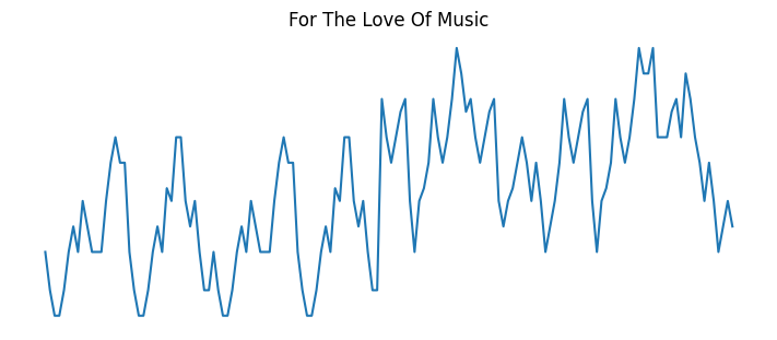
Trajectory

Something simple we can do is plot the trajectory, as a sort of time series. Ignoring note duration, that looks like this:

y = np.array([n.value for n in tune.iter_notes()])
x = np.arange(len(y)) * 1/8

plt.figure(figsize=(7, 3), layout="constrained")
plt.axis("off")
plt.title(tune.title)
plt.plot(x, y);

Or, considering duration:

plt.figure(figsize=(7, 3), layout="constrained")

y = np.array([n.value for n in tune.iter_notes()])
x = np.arange(1, len(y) + 1) * 1/8  # shift for consistency

plt.plot(x, y, label="ignored")

data = np.array(
    [
        [n.value, float(n.duration)]
        for n in tune.iter_notes()
    ]
)
x = data[:,1].cumsum()  # ends of notes
y = data[:,0]
assert len(x) == len(y)

plt.plot(x, y, label="considered")
plt.axis("off")
plt.title(tune.title)
plt.legend(title="duration", loc="upper left");

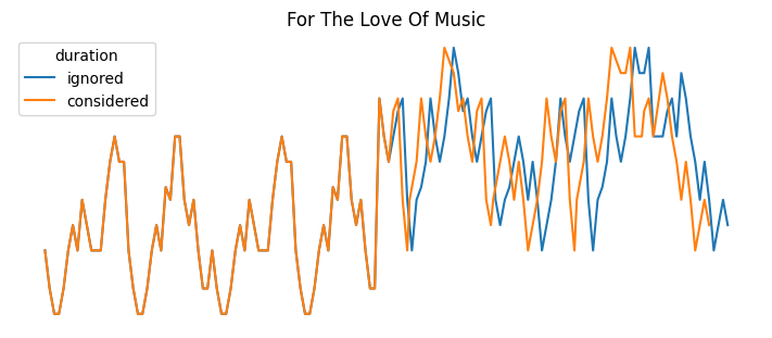
The divergence occurs due to the 16th notes in the B part.

Histogram

We can make a histogram of the notes, again considering duration or not.

data = [
    [n.value, float(n.duration), n.to_pitch().unicode()]
    for n in tune.iter_notes()
]

df = pd.DataFrame(data, columns=["value", "duration", "pitch"])

_, ax = plt.subplots(figsize=(6, 3.5), layout="constrained")

count = (
    df.groupby("value")
    .aggregate({"pitch": "first", "duration": "size"})
    .rename(columns={"duration": "unweighted"})
    .assign(
        weighted=(
            df.assign(w=df["duration"] * 8)
            .groupby("value")["w"].sum()
        )
    )
)

count.plot.bar(
    x="pitch",
    rot=0,
    xlabel="Pitch",
    ylabel="Count",
    title=tune.title,
    ax=ax,
);

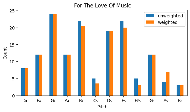
Note

F♯₄ is skipped in this plot, which is a bit misleading. It would be better to have an empty place for it.

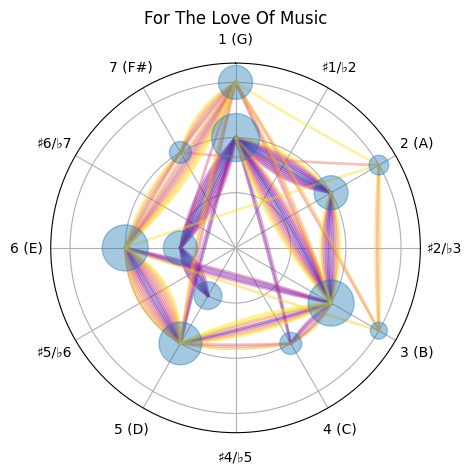
Polar

We can combine the two (trajectory and histogram) in a polar plot (featured in the readme).

Some tools Hide code cell content

def quadratic_bezier(p1, p2, p3, *, n=200):
    """Quadratic Bezier curve from start, middle, and end points."""
    # based on https://stackoverflow.com/a/61385858

    (xa, ya), (xb, yb), (xc, yc) = p1, p2, p3

    def rect(x1, y1, x2, y2):
        a = (y1 - y2) / (x1 - x2)
        b = y1 - a * x1
        return (a, b)

    x1, y1, x2, y2 = xa, ya, xb, yb
    a1, b1 = rect(xa, ya, xb, yb)
    a2, b2 = rect(xb, yb, xc, yc)

    x = np.full((n,), np.nan)
    y = x.copy()
    for i in range(n):
        a, b = rect(x1, y1, x2, y2)

        x[i] = i*(x2 - x1)/n + x1
        y[i] = a*x[i] + b

        x1 += (xb - xa)/n
        y1 = a1*x1 + b1
        x2 += (xc - xb)/n
        y2 = a2*x2 + b2

    return x, y


def get_polar_ax(key):
    from pyabc2 import PitchClass

    _, ax = plt.subplots(subplot_kw={"projection": "polar"})

    chromatic_scale_degrees = np.arange(12)
    note_labels = []
    for csd in chromatic_scale_degrees:
        pc = PitchClass(csd + key.tonic.value)
        sd = pc.scale_degree_in(key, acc_fmt="unicode")
        if pc in key.scale:
            s = f"{sd} ({pc.name})"
        else:
            s = sd
        note_labels.append(s)

    ax.set_theta_offset(np.pi/2)
    ax.set_theta_direction(-1)
    ax.set_xticks(chromatic_scale_degrees/12 * 2*np.pi)
    ax.set_xticklabels(note_labels)
    ax.set_rlabel_position(225)  # deg.
    ax.xaxis.set_tick_params(pad=7)
    ax.set_rlim(0, 3.35)  # TODO: configurable (and/or based on Tune)
    ax.set_rticks([1, 2, 3])
    ax.set_yticklabels([])

    return ax

from collections import Counter

from pyabc2 import Pitch

ref = Pitch.from_name("G4")

# Compute relative pitch values
v = [n.value - ref.value for n in tune.iter_notes()]
v = np.array(v)

# Set up ax
ax = get_polar_ax(tune.key)
ax.set_title(tune.title)

# Compute and plot trajectory
r0, v0 = np.divmod(v, 12)
# TODO: try spiral-y version with continuous r (v/12)
r = r0 - r0.min() + 1
t = v0 * 2 * np.pi / 12
cmap = plt.get_cmap("plasma")
colors = [cmap(x) for x in np.linspace(0, 1, len(r) - 1)]
traj_count = Counter()
for c, t1, r1, t2, r2 in zip(colors[:], t[:-1], r[:-1], t[1:], r[1:]):
    p1, p3 = (r1*np.cos(t1), r1*np.sin(t1)), (r2*np.cos(t2), r2*np.sin(t2))
    if p1 == p3:
        continue

    traj = ((t1, r1), (t2, r2))
    traj_count[traj] += 1

    # Calculate isos triangle vertex point
    # (to move the traj line out of the way of previous same motions)
    mx = (p1[0] + p3[0]) / 2
    my = (p1[1] + p3[1]) / 2
    mt = np.arctan2(p3[1] - p1[1], p3[0] - p1[0])
    h = 0.05 + 0.07 * (traj_count[traj] - 1)
    # TODO: ^ would be nice to know total count beforehand, so to set a max for h
    p2 = (mx + h*np.cos(mt - np.pi/2), my + h*np.sin(mt - np.pi/2))

    # Plot Bezier curve
    xb, yb = quadratic_bezier(p1, p2, p3)
    rb = np.sqrt(xb**2 + yb**2)
    tb = np.arctan2(yb, xb)
    ax.plot(tb, rb, c=c, lw=2, alpha=0.4)

# Compute and plot histogram data
# TODO: optionally weight with duration
vc = Counter(v)
rc0, vc0 = np.divmod(list(vc), 12)
rc = rc0 - rc0.min() + 1
tc = vc0 * 2 * np.pi / 12
s = np.array(list(vc.values())) * 50
ax.scatter(
    tc,
    rc,
    s=s,
    marker="o",
    zorder=10,
    alpha=0.4,
);